In this article, we focused on using regression to predict a continuous value house prices from features of the house (e.g. square feet of living space, number of bedrooms,...). In this IPython Notebook, we are going to build a more accurate regression model for predicting house prices by including more features of the house. During this process, we are also going familiar with how the Python language can be used for data exploration .!
graphlab.product_key.set_product_key()
# CSV format data https://d396qusza40orc.cloudfront.net/phoenixassets/home_data.csv
sales = graphlab.SFrame('coursera-notebooks/course-1/home_data.gl')
[INFO] This non-commercial license of GraphLab Create is assigned to prashantgonarkar@gmail.com and will expire on February 13, 2017. For commercial licensing options, visit https://dato.com/buy/.

[INFO] Start server at: ipc:///tmp/graphlab_server-1182 - Server binary: /usr/local/lib/python2.7/dist-packages/graphlab/unity_server - Server log: /tmp/graphlab_server_1455457362.log
[INFO] GraphLab Server Version: 1.8
| id |
date |
price |
bedrooms |
bathrooms |
sqft_living |
sqft_lot |
floors |
waterfront |
| 7129300520 |
2014-10-13 00:00:00+00:00 |
221900 |
3 |
1 |
1180 |
5650 |
1 |
0 |
| 6414100192 |
2014-12-09 00:00:00+00:00 |
538000 |
3 |
2.25 |
2570 |
7242 |
2 |
0 |
| 5631500400 |
2015-02-25 00:00:00+00:00 |
180000 |
2 |
1 |
770 |
10000 |
1 |
0 |
| 2487200875 |
2014-12-09 00:00:00+00:00 |
604000 |
4 |
3 |
1960 |
5000 |
1 |
0 |
| 1954400510 |
2015-02-18 00:00:00+00:00 |
510000 |
3 |
2 |
1680 |
8080 |
1 |
0 |
| 7237550310 |
2014-05-12 00:00:00+00:00 |
1225000 |
4 |
4.5 |
5420 |
101930 |
1 |
0 |
| 1321400060 |
2014-06-27 00:00:00+00:00 |
257500 |
3 |
2.25 |
1715 |
6819 |
2 |
0 |
| 2008000270 |
2015-01-15 00:00:00+00:00 |
291850 |
3 |
1.5 |
1060 |
9711 |
1 |
0 |
| 2414600126 |
2015-04-15 00:00:00+00:00 |
229500 |
3 |
1 |
1780 |
7470 |
1 |
0 |
| 3793500160 |
2015-03-12 00:00:00+00:00 |
323000 |
3 |
2.5 |
1890 |
6560 |
2 |
0 |
| view |
condition |
grade |
sqft_above |
sqft_basement |
yr_built |
yr_renovated |
zipcode |
lat |
| 0 |
3 |
7 |
1180 |
0 |
1955 |
0 |
98178 |
47.51123398 |
| 0 |
3 |
7 |
2170 |
400 |
1951 |
1991 |
98125 |
47.72102274 |
| 0 |
3 |
6 |
770 |
0 |
1933 |
0 |
98028 |
47.73792661 |
| 0 |
5 |
7 |
1050 |
910 |
1965 |
0 |
98136 |
47.52082 |
| 0 |
3 |
8 |
1680 |
0 |
1987 |
0 |
98074 |
47.61681228 |
| 0 |
3 |
11 |
3890 |
1530 |
2001 |
0 |
98053 |
47.65611835 |
| 0 |
3 |
7 |
1715 |
0 |
1995 |
0 |
98003 |
47.30972002 |
| 0 |
3 |
7 |
1060 |
0 |
1963 |
0 |
98198 |
47.40949984 |
| 0 |
3 |
7 |
1050 |
730 |
1960 |
0 |
98146 |
47.51229381 |
| 0 |
3 |
7 |
1890 |
0 |
2003 |
0 |
98038 |
47.36840673 |
| long |
sqft_living15 |
sqft_lot15 |
| -122.25677536 |
1340.0 |
5650.0 |
| -122.3188624 |
1690.0 |
7639.0 |
| -122.23319601 |
2720.0 |
8062.0 |
| -122.39318505 |
1360.0 |
5000.0 |
| -122.04490059 |
1800.0 |
7503.0 |
| -122.00528655 |
4760.0 |
101930.0 |
| -122.32704857 |
2238.0 |
6819.0 |
| -122.31457273 |
1650.0 |
9711.0 |
| -122.33659507 |
1780.0 |
8113.0 |
| -122.0308176 |
2390.0 |
7570.0 |
[21613 rows x 21 columns]
Note: Only the head of the SFrame is printed.
You can use print_rows(num_rows=m, num_columns=n) to print more rows and columns.
Exploring the data
graphlab.canvas.set_target('ipynb')
sales.show(view="Scatter Plot",x="sqft_living",y="price")
Create simple regression model of sqft_livingto price
train_data,test_data = sales.random_split(.8,seed=471829)
Build the regression model
sqft_model = graphlab.linear_regression.create(train_data,target='price',features=['sqft_living'])
PROGRESS: Creating a validation set from 5 percent of training data. This may take a while.
          You can set ``validation_set=None`` to disable validation tracking.

PROGRESS: Linear regression:
PROGRESS: --------------------------------------------------------
PROGRESS: Number of examples          : 16319
PROGRESS: Number of features          : 1
PROGRESS: Number of unpacked features : 1
PROGRESS: Number of coefficients    : 2
PROGRESS: Starting Newton Method
PROGRESS: --------------------------------------------------------
PROGRESS: +-----------+----------+--------------+--------------------+----------------------+---------------+-----------------+
PROGRESS: | Iteration | Passes   | Elapsed Time | Training-max_error | Validation-max_error | Training-rmse | Validation-rmse |
PROGRESS: +-----------+----------+--------------+--------------------+----------------------+---------------+-----------------+
PROGRESS: | 1         | 2        | 1.003736     | 4333270.446305     | 2128076.109406       | 263914.025655 | 245344.423754   |
PROGRESS: +-----------+----------+--------------+--------------------+----------------------+---------------+-----------------+
PROGRESS: SUCCESS: Optimal solution found.
PROGRESS:
Evaluate simple model
print test_data['price'].mean()
sqft_model.evaluate(test_data)
{'max_error': 3254412.8838123637, 'rmse': 255356.74724801505}
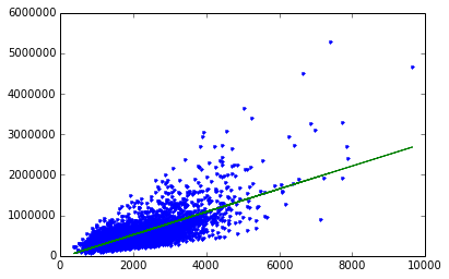
Let's show what our predictions look like
import matplotlib.pyplot as plt
%matplotlib inline
plt.plot(test_data['sqft_living'],test_data['price'],'.',
         test_data['sqft_living'],sqft_model.predict(test_data),'-')
[<matplotlib.lines.Line2D at 0x7f0e4c130390>,
 <matplotlib.lines.Line2D at 0x7f0e70d7c650>]
sqft_model.get('coefficients')
| name |
index |
value |
stderr |
| (intercept) |
None |
-49529.3244096 |
5126.67769256 |
| sqft_living |
None |
283.506960839 |
2.25772750653 |
[2 rows x 4 columns]
Explore other features in the data
my_features = ['bedrooms','bathrooms','sqft_living','sqft_lot','floors','zipcode']
sales[my_features].show()
sales.show(view="BoxWhisker Plot",x='zipcode',y='price')
Build a regression model with more number of features
my_feature_model = graphlab.linear_regression.create(train_data,target='price',features=my_features)
PROGRESS: Creating a validation set from 5 percent of training data. This may take a while.
          You can set ``validation_set=None`` to disable validation tracking.

PROGRESS: Linear regression:
PROGRESS: --------------------------------------------------------
PROGRESS: Number of examples          : 16367
PROGRESS: Number of features          : 6
PROGRESS: Number of unpacked features : 6
PROGRESS: Number of coefficients    : 118
PROGRESS: Starting Newton Method
PROGRESS: --------------------------------------------------------
PROGRESS: +-----------+----------+--------------+--------------------+----------------------+---------------+-----------------+
PROGRESS: | Iteration | Passes   | Elapsed Time | Training-max_error | Validation-max_error | Training-rmse | Validation-rmse |
PROGRESS: +-----------+----------+--------------+--------------------+----------------------+---------------+-----------------+
PROGRESS: | 1         | 2        | 0.037789     | 3769052.655633     | 1309832.673966       | 180398.263404 | 157403.059497   |
PROGRESS: +-----------+----------+--------------+--------------------+----------------------+---------------+-----------------+
PROGRESS: SUCCESS: Optimal solution found.
PROGRESS:
['bedrooms', 'bathrooms', 'sqft_living', 'sqft_lot', 'floors', 'zipcode']
print sqft_model.evaluate(test_data)
print my_feature_model.evaluate(test_data)
{'max_error': 3254412.8838123637, 'rmse': 255356.74724801505}
{'max_error': 2589520.1383550493, 'rmse': 184401.4046152276}
Apply learned model to predict prices of 3 houses
house1 = sales[sales['id']=='5309101200']
| id |
date |
price |
bedrooms |
bathrooms |
sqft_living |
sqft_lot |
floors |
waterfront |
| 5309101200 |
2014-06-05 00:00:00+00:00 |
620000 |
4 |
2.25 |
2400 |
5350 |
1.5 |
0 |
| view |
condition |
grade |
sqft_above |
sqft_basement |
yr_built |
yr_renovated |
zipcode |
lat |
| 0 |
4 |
7 |
1460 |
940 |
1929 |
0 |
98117 |
47.67632376 |
| long |
sqft_living15 |
sqft_lot15 |
| -122.37010126 |
1250.0 |
4880.0 |
[? rows x 21 columns]
Note: Only the head of the SFrame is printed. This SFrame is lazily evaluated.
You can use len(sf) to force materialization.
print sqft_model.predict(house1)
print my_feature_model.predict(house1)
## Prediction for second fancier house
house2 = sales[sales['id'] == '1925069082']
| id |
date |
price |
bedrooms |
bathrooms |
sqft_living |
sqft_lot |
floors |
waterfront |
| 1925069082 |
2015-05-11 00:00:00+00:00 |
2200000 |
5 |
4.25 |
4640 |
22703 |
2 |
1 |
| view |
condition |
grade |
sqft_above |
sqft_basement |
yr_built |
yr_renovated |
zipcode |
lat |
| 4 |
5 |
8 |
2860 |
1780 |
1952 |
0 |
98052 |
47.63925783 |
| long |
sqft_living15 |
sqft_lot15 |
| -122.09722322 |
3140.0 |
14200.0 |
[? rows x 21 columns]
Note: Only the head of the SFrame is printed. This SFrame is lazily evaluated.
You can use len(sf) to force materialization.
print sqft_model.predict(house2)
print my_feature_model.predict(house2)
last house, super fancy
bill_gates = {'bedrooms':[8],
              'bathrooms':[25],
              'sqft_living':[50000],
              'sqft_lot':[225000],
              'floors':[4],
              'zipcode':['98039'],
              'condition':[10],
              'grade':[10],
              'waterfront':[1],
              'view':[4],
              'sqft_above':[37500],
              'sqft_basement':[12500],
              'yr_built':[1994],
              'yr_renovated':[2010],
              'lat':[47.627606],
              'long':[-122.242054],
              'sqft_living15':[5000],
              'sqft_lot15':[40000]}
print my_feature_model.predict(graphlab.SFrame(bill_gates))
Selection and summary statistics
dtype: str
Rows: 21613
['98178', '98125', '98028', '98136', '98074', '98053', '98003', '98198', '98146', '98038', '98007', '98115', '98028', '98074', '98107', '98126', '98019', '98103', '98002', '98003', '98133', '98040', '98092', '98030', '98030', '98002', '98119', '98112', '98115', '98052', '98027', '98133', '98117', '98117', '98058', '98115', '98052', '98107', '98001', '98056', '98074', '98166', '98053', '98119', '98058', '98019', '98023', '98007', '98115', '98070', '98148', '98056', '98117', '98117', '98105', '98105', '98042', '98042', '98008', '98059', '98166', '98148', '98166', '98115', '98122', '98144', '98004', '98001', '98042', '98004', '98005', '98034', '98125', '98038', '98042', '98075', '98008', '98116', '98133', '98010', '98038', '98038', '98118', '98059', '98125', '98119', '98092', '98056', '98056', '98136', '98023', '98199', '98023', '98117', '98117', '98040', '98032', '98023', '98038', '98045', ... ]
temp_zipcode = sales[sales['zipcode']=='98039']
temp_zipcode['price'].mean()
Filtering data using SFrame
num_houses = sales[(sales['sqft_living'] > 2000) & (sales['sqft_living'] < 4000) ]
total_houses = sales.num_rows()
required_houses = num_houses.num_rows()
float(required_houses) / float(total_houses)
Building a regression model with several more features
advanced_features = [
'bedrooms', 'bathrooms', 'sqft_living', 'sqft_lot', 'floors', 'zipcode',
'condition', # condition of house
'grade', # measure of quality of construction
'waterfront', # waterfront property
'view', # type of view
'sqft_above', # square feet above ground
'sqft_basement', # square feet in basement
'yr_built', # the year built
'yr_renovated', # the year renovated
'lat', 'long', # the lat-long of the parcel
'sqft_living15', # average sq.ft. of 15 nearest neighbors
'sqft_lot15', # average lot size of 15 nearest neighbors
]
train_data,test_data = sales.random_split(.8,seed=0)
['bedrooms', 'bathrooms', 'sqft_living', 'sqft_lot', 'floors', 'zipcode']
my_features_model = graphlab.linear_regression.create(train_data,target='price',features=my_features,validation_set=None)
PROGRESS: Linear regression:
PROGRESS: --------------------------------------------------------
PROGRESS: Number of examples          : 17384
PROGRESS: Number of features          : 6
PROGRESS: Number of unpacked features : 6
PROGRESS: Number of coefficients    : 115
PROGRESS: Starting Newton Method
PROGRESS: --------------------------------------------------------
PROGRESS: +-----------+----------+--------------+--------------------+---------------+
PROGRESS: | Iteration | Passes   | Elapsed Time | Training-max_error | Training-rmse |
PROGRESS: +-----------+----------+--------------+--------------------+---------------+
PROGRESS: | 1         | 2        | 0.034821     | 3763208.270524     | 181908.848367 |
PROGRESS: +-----------+----------+--------------+--------------------+---------------+
PROGRESS: SUCCESS: Optimal solution found.
PROGRESS:
print my_features_model.evaluate(test_data)
{'max_error': 3486584.5093818563, 'rmse': 179542.4333126908}
my_advanced_model = graphlab.linear_regression.create(train_data,target='price',features=advanced_features,validation_set=None)
PROGRESS: Linear regression:
PROGRESS: --------------------------------------------------------
PROGRESS: Number of examples          : 17384
PROGRESS: Number of features          : 18
PROGRESS: Number of unpacked features : 18
PROGRESS: Number of coefficients    : 127
PROGRESS: Starting Newton Method
PROGRESS: --------------------------------------------------------
PROGRESS: +-----------+----------+--------------+--------------------+---------------+
PROGRESS: | Iteration | Passes   | Elapsed Time | Training-max_error | Training-rmse |
PROGRESS: +-----------+----------+--------------+--------------------+---------------+
PROGRESS: | 1         | 2        | 0.087034     | 3469012.450487     | 154580.940732 |
PROGRESS: | 2         | 3        | 0.145169     | 3469012.450673     | 154580.940735 |
PROGRESS: +-----------+----------+--------------+--------------------+---------------+
PROGRESS: SUCCESS: Optimal solution found.
PROGRESS:
print my_advanced_model.evaluate(test_data)
{'max_error': 3556849.4138490623, 'rmse': 156831.11680200786}
Credits Machine Learning Foundations: A Case Study Approach